Affiliate links on Android Authority may earn us a commission. Learn more.
How to add error bars in Excel
Published onMarch 1, 2023
If you use Excel to create charts, it’s always good to know what customization options you have for your data entries. Excel allows you to display all sorts of data and possible variations. Error bars can aid you in displaying margins of error or standard deviations within your data. Let’s go over how to add error bars in Excel.
QUICK ANSWER
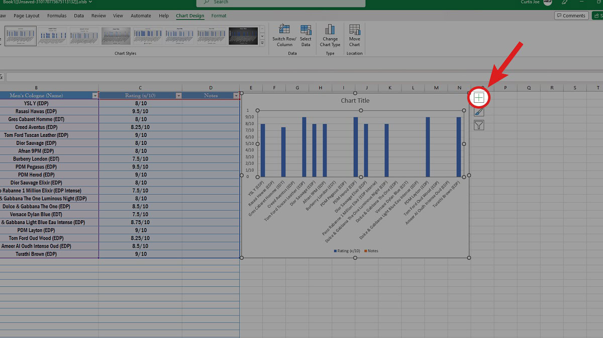
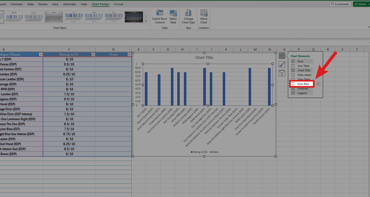
To add error bars in Excel, click on your chart or graph in Excel. Click Chart Elements > Error Bars.
How to add error bars in Excel
Using the data in your Excel spreadsheet, create a chart. Click the chart, then click the Chart Elements (+) button to its right.

A selection of chart elements will appear in a smaller menu. From the options available, click Error Bars.
If you click the arrow to its right, an extended menu will reveal Standard Error, Percentage, Standard Deviation, and More Options…. You can use these to further customize your error bars.

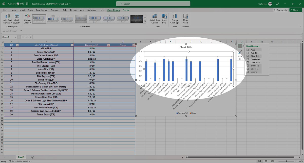
When finished, your chart will display error bars on your data points.

FAQs
Typically, for charts and graphs, error bars will appear as an option from the Chart Elements extended menu. However, if it doesn’t appear, there’s a chance you’re working with a 3D chart. These don’t allow you to add error bars.