How to sum and subtract in Google Sheets

Did you know that your spreadsheet can double as a calculator? Google Sheets has various functions that do the math for you, which is especially helpful when handling large data sets. As with learning anything, it’s best to start with the basics. Here’s how to sum and subtract in Google Sheets.

How to sum in Google Sheets

Adding up columns or rows of numbers is familiar to most spreadsheet programs. Google Sheets includes a built-in function named SUM to add the total value. There are two easy ways to utilize the SUM function.

Typing the SUM function:

• Click on the cell where you want the sum to be displayed.
• Type =SUM( (make sure to include the equal sign).
• You can then select the cells you want to add directly by clicking and dragging on them in the sheet.
• Alternatively, you can type the cell references manually separated by commas (e.g., =SUM(A1,B1,C1)).

• Close the parenthesis and press Enter. Google Sheets will automatically calculate the sum.

Using Sum in Functions:

• Highlight the cells where you want to sum.
• Locate the Functions button (Σ) on the toolbar.
• Choose SUM, Google Sheets will sum the range you want based on the highlighted cells.
• If the selection is correct, press Enter to confirm. If not, adjust the range directly in the formula bar before pressing Enter.

Both methods achieve the same result. The sum can be quicker for simple sums, but typing the formula method gives you more control over the specific cells being added.

Here are some additional points to keep in mind:

• • The SUM function can also handle ranges of cells. For example, =SUM(A1:A10)will add all the values from cells A1 to A10.
  • You can also include other cells or functions within the SUM function for more complex calculations.

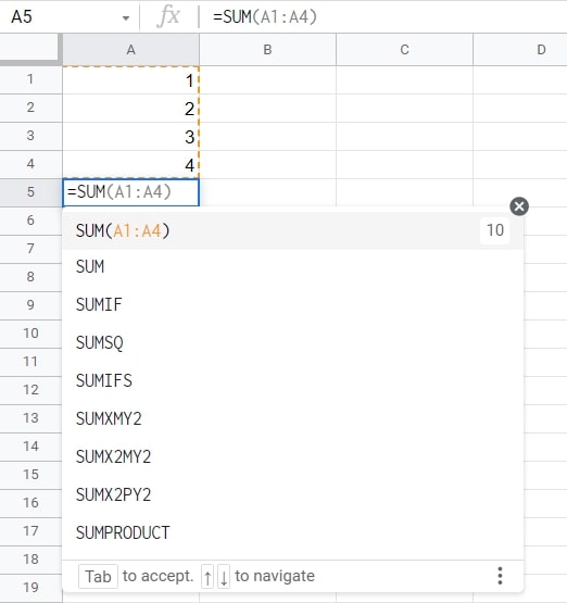
You will notice that the function will preview the result in a small pop-up window, in this case, 10. When ready to sum, hit the Enter key, and the function result will appear in the cell.

How to subtract in Google Sheets

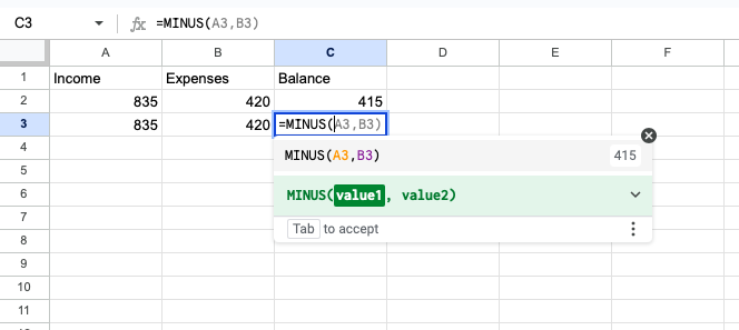
As with summing, subtracting can be done in two easy ways. For this example, we’ll subtract each expenditure value (column B) from each income value (column A) and place the resulting balance in column C.

Using the minus sign (-):

• Click on the cell where you want the difference displayed.
• Type the equal sign (=) to initiate the formula. This will cause Google Sheets to suggest the numbers to the left as input values, which you can select by pressing Tab.
• Click on the cell with the first number you want to subtract.
• Then, type the minus sign (-).
• Finally, enter the second number you want to subtract or click on the cell containing it.
• Press Enter and Google Sheets will show the difference.

For example, if you want to subtract the value in cell B2 from the value in cell A2, you would enter =A2-B2 in the formula bar.

Next, the difference is displayed in cell C2, and you’ll notice a small blue square in the bottom right corner. This is called the Fill Handle, and it’s pretty handy.

• You can click and drag the fill handle down the rest of the column to quickly subtract the remaining values.
• Then, release the left-click on your mouse, and the differences in each row’s values will be displayed down the column. This saves you time from writing the function over and over.

Using the MINUS function:

• While not necessary, Google Sheets also offers a MINUS function, which essentially does the same thing as the minus sign. You can find the function from the Insert tab or type it in the cell as =MINUS.
• The syntax is =MINUS(value1, value2).
• Replace value1 and value2 with the numbers you want to subtract or references to the cells containing them.

As with the previous example, you can click and drag the Fill Handle to apply the function to the rest of the rows.

Both methods achieve the same result. The minus sign is generally quicker for simple subtractions, while the MINUS function might be useful if you’re working within a larger formula and prefer to use functions for consistency.

Here are some additional tips for subtracting in Google Sheets:

• You can subtract multiple cells from a single value. For example, to subtract values in cells B3 and B4 from the value in A3, you would use =A3-SUM(B3:B4).
• You can use cell references to ensure your formulas update automatically when the original values change.

How to solve errors when adding and subtracting in Google Sheets

Whenever you enter a formula into a cell, and the spreadsheet software cannot understand what you want it to do, we call that a parse error. The two common causes for this error are a typo in your formula or unclear order of operations. For example, typing =+ instead of =, forgetting to put quotation marks around text values, or leaving out parentheses are all things we can easily miss.

Here’s a list of errors and why your formulas might not work correctly.

• #N/A Error: One of the most common errors is when a formula can’t find what it’s looking for. Check your formula inputs and make sure they’re correct.
• #DIV/0 Error: This happens when you try to divide a number by zero. Don’t do that.
• #REF! Error: You will get this error message when a formula contains an invalid cell reference; for example, if you have a formula that references cells B15:B25 and delete row 24, the formula will return the #REF! Error because it no longer has a valid reference.
• #VALUE Error: This error occurs when a formula contains an invalid value. For example, if you have a formula that adds two cells and one of the cells contains text instead of a number, you’ll get this error.
• #NAME Error: This error occurs when a formula contains an invalid name. For example, if you have a named range called “Expenses” and accidentally type “s” at the end of your formula, you’ll get the #NAME? error
• #NUM Error: The #NUM! error occurs when a formula contains an invalid number. This can happen when a formula is applied to two or more cells, and the result is too large to display.

Double-check your formula inputs and ensure you’re using the correct operators.

FAQs